Change Excel Color Scheme (Skin Color)

How to change skin of my Excel 2007?
HINT: Use Excel Options then Color Scheme

You can change your Excel 2007 color scheme with Blue, Silver, or Black.


Black color scheme:

















Blue color scheme:

















Silver color scheme:





Step 01:
Click Office button.





Step 02:
Click Excel Options.

























Step 03:
On Popular, change Color Scheme to Blue, Silver, or Black.
Then press OK button.

Open your 2007 excel files on Excel 2003

I can't open file excel 2007 on my MS Excel 2003
HINT: Install Compatibility Pack












Install from this link !!!
Then you can open your excel 2007 file on your MS Excel 2003 or later !!!

Subtotal your values

How to calculate subtotal?
HINT: Use SUM function


















Step 01:
Type your data

Step 02:
Select your subtotal cell




Step 03:
Type "=SUM(" then select your data, then press ENTER
In this case, my data are from F4 to F14 (F4:F14), so you see "=SUM(F4:F14)" in formula bar.

Create Chart with Fast

How to create chart with Fast?
HINT: Use shortcut Alt-F1

Step 01:
Select your data





















Step 02:
Press Alt-F1 and voila.. you got a column chart !!!

Change Horizontal Axis chart

How to change horizontal axis chart on Excel 2007?
HINT: Use Select Data




















Step 01:
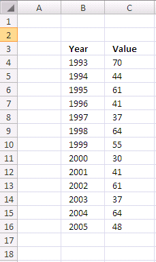
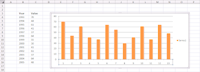
Type your data chart and type also your new axis label.
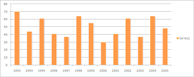
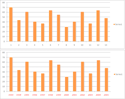
I will change horizontal axis label (1,2,3,....13) to 1993,1994,1995,...,2005























Step 02:
Now, click on label number exactly (example click horizontal axis label 7). Then you will see all horizontal axis label selected.










Step 03:
After that, right-click it and then you will see the menu. Click Select Data...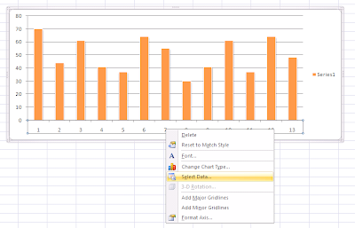
















Step 04:
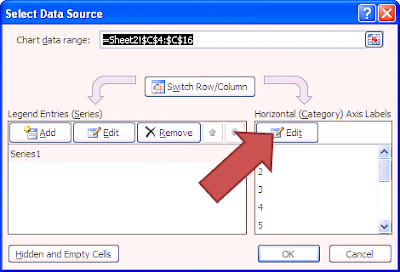
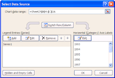
The Select Data Source window will appear. Select right Edit button (see picture):

















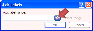
Step 05:
Axis Labels window appear. Click the range button (see picture):








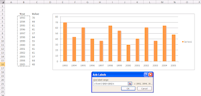
Step 06:
Select your new axis label. In this case, I select Year column.
Selected cells will marked like ants march. If you done, click OK button.













Step 07:
The Select Data Source window will appear again. See that Horizontal (Category) Axis Labels now 1993, 1994, ......, 2005. Click OK button to finish it.

















Step 08:
Now, you will see your horizontal axis label will change to year.

Insert Symbol

How to insert a symbol to Excel 2007?
HINT: Use Insert | Symbol

for example, I need to insert a check mark symbol to my cell






Step 01:
Click Insert tab then select Symbol





Step 02:
The Symbol window will appear. In the Font dropdown list, select Wingdings font.



















Step 03:
Wingding font will display its font members !



















Step 04:
To search check mark symbol, keep scrolling down until you find the check mark symbol.



















Step 05:
After you find it, click it then click Insert button then click Close button if you want to close the window.

Show Developer tab

How to show Developer tab?
HINT: Use Excel Options


Step 01:
Click Office Button





Step 02:
Click Excel Options
























Step 03:
On Popular, tick Show Developer tab in the Ribbon. Then click OK button.

Phone Number format

How to change 6038017144 into (603)801-7144 ?
HINT: Use Format Cells...





There is two way to do this.
1. Using Format Cells... | Special | Phone number, or
2. Using Format Cells... | Custom | (###) ###-####

Using Special | Phone number
Step 01:
Type your number then select it

Step 02:
Right-click the cell then click Format Cells...


















Step 03:
Select Special, then select Phone number. Click OK button.

























Using Format Cells... | Custom | (###) ###-####

Step 01:
Type your number then select it

Step 02:
Right-click the cell then click Format Cells...


















Step 03:
Select Custom, then type (###) ###-####. Click OK button.

Linear Regression with Excel

How to plot Linear Regression on Excel?
HINT: Use Trendline on your scatter chart

Step 01
Type your data on Excel cells













Step 02
Select all y data value (not x)














Step 03
Click Insert menu, then select Scatter chart type. Select one type.














Step 04
Now you get your scatter chart











Step 05
Click on data plot (exactly on one of the blue dots) so they selected. Then right click the selected to show the menu. Click on the Add Trendline...

















Step 06
Choose Linear on the Trend/Regression Type.
Choose Display Equation on Chart.
Choose Display R-squared value on chart.
























Step 07
Finally you got Linear Regression

Clear Recent Files

To clear the list of recently used files in Excel 2007, you have to restrict the list to no entries. To do this, follow these steps:

Step 01:
Click the Microsoft Office Button, and then click Excel Options.






Step 02:
In the left pane, click Advanced




















... keep scrolling down after you see this (Show this number of Recent Documents) :











Step 03:
Under Display, type 0 in the Show this number of Recent Documents box, then press OK button.


After you follow these steps, a list of recently used files will not be displayed. If you want a list of recently used files to be displayed again, repeat steps 2 through 3. Then, type a number other than 0 in the Show this number of Recent Documents box.

from: http://support.microsoft.com/kb/926535

Create Drop down List

How to create Dropdown list?
HINT: Use Validation Data feature

Step 01:
Create the item list on sheet1











Step 02:
I will create new name range, so this list I can use in other sheet





















Step 03:
Type your data range name ( I name it with "ItemList") then press Enter.





















Step 04:
Move to other sheet (for example, I move to sheet2).
Select cell B2 (for example), then select Data menu, then click Data Validation...









Step 05:
Data Validation window appear. Then select List from Validation Criteria.




















Step 06:
Fill Source with "=ItemList" then press OK button




















Step 07:
Now your cell already have dropdown list








Step 08:
Click on the dropdown list button to choose your data